Counting Number of Queries Executed in SSAS

When monitoring SSAS we can use a few tools to gain insight into what is happening on the instance. Perfmon is especially interesting as it shows us information about various aspects of the server – we can see memory, disk, CPU and MDX counters out of the box. However, perfmon cannot show us how many queries were run on SSAS – neither per period (e.g. second), nor in total since the service had started. We have another counter, similar to a count of queries – Storage Engine Query : Total Queries Answered. This is not the same as the number of MDX queries answered, as if a query does not hit the Storage Engine (SE), but the Formula Engine (FE) cache instead, it won’t increment the counter. And, if a query needs to be answered by more than one Storage Engine requests, we will see that the counter gets incremented with more than 1.

There are alternatives. We can try using the Query Log server settings and save queries to a database table automatically:

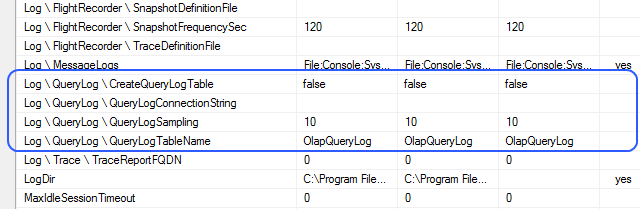
Unfortunately (for us in this case), since the Query Log is typically used for Usage Based Optimisations (UBO), it also shows SE requests, not the actual MDX queries issued. Hence, it suffers from the same drawback as the perfmon Total Queries Answered counter.

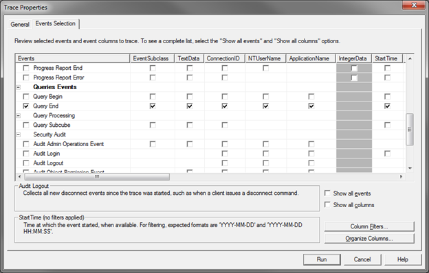
The other alternative which comes to mind is SQL Server Profiler. After all it allows us to see what queries get sent to the server, along with lots of other useful information. If we are interested in the count of queries only, we can capture a trace which includes only the Query End event. Why not Query Begin? Well, we can’t see some possibly interesting numbers before the query has been executed, for example the Duration of each query. If we capture only Query End we get exactly what we need – one event per query. We can also capture Error events to check if things go wrong.

A typical Query End-only trace looks like this (all columns included):

As we can see above, we get the actual query in the TextData column, the User Name, Application Name, Duration, Database Name – all very useful properties if we want to analyse the load and the performance of our server and various solutions. While the information looks great on screen, having it in a database table would enable us to do what we (BI devs) like doing – play with the data. Only this time it’s our data, about our toys, so it (at least for me) is twice as fun.

A SSAS trace can be run on the server without Profiler – the term for it is a “server-side trace”. Unlike SQL Server RDBMS traces, a SSAS server-side trace cannot directly log its output to a SQL Server table. Luckily, we can write the results in a “.trc” file, which in turn can be imported into a SQL Server table with a few lines of code.

To create a server-side trace we can first export the trace definition to an XMLA file from profiler:

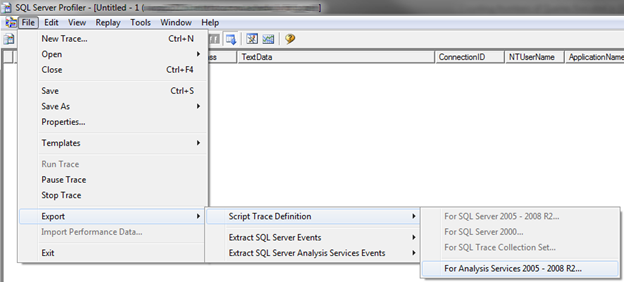
The XMLA file we get looks like this (all scripts are attached to the end of this post):

If we remove the first line (?xml version…), we can run this and it will create a trace on the server. This trace is useless to us because it does not write its output anywhere. To fix this we can add a few settings like this:

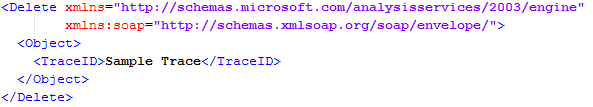
Note that I have changed the Name and ID of the trace to be more user-friendly, and I have removed the Filers section, as well as the first line. Now the script can be used to create a trace. To delete the trace we can use:

And to list all running traces on a SSAS instance:

Note that by default SSAS is configured to run Flight Recorder, which uses a trace to capture events happening on the server (thanks to Dan English for suggesting this clarification). The trace may appear with ID and Name of FlightRecorder. You should not tamper with the trace manually. If you want to stop it, which is a performance recommendation from the SSAS Performance Guide, you should disable Flight Recorder from the SSAS server properties (click for a larger version):

Now, armed with all these scripts we can effectively manage traces on our instances. The only problem we have not resolved so far is exporting the trc file created by our create trace XMLA command to a database table. This can be easily done in a .NET app, or in PowerShell. The ps_trace_copy_to_table.ps1 PowerShell script does the following (thanks to Darren Gosbell for creating the initial version).

1. Copy the trc file with another name for further processing
2. Delete the trace form the server
3. Delete the trace file
4. Start the trace on the server again
5. Export the copied trc file into a SQL Server table
6. Run a stored procedure moving the data from the SQL Server table to another SQL Server table which contains all trace data

We delete->create the trace because otherwise we cannot delete the trace file. The last step runs a stored procedure which moves the data from the table we imported into to another table because the first (landing) table gets re-created every time we import into it and the trace data cannot persist in it.

Note that there is some exception handling implemented in this script (try/catch/finally blocks). If you are using an old version of PowerShell, it is possible that you may have to remove the exception handling statements as they were not supported. I have attached a sample script which excludes them (ps_trace_copy_to_table_no_exception_handling.ps1).

Finally, we can run this script through SQL Server Agent on regular intervals. SQL Server Agent allows direct PowerShell script execution, so this is very easy to set up and can be scheduled to run recurrently every X minutes/hours/days.

A small note: you may notice that some rows in the database table contain events with an Event Class <> 10 (10 is Query End) and NULLs in most columns. These are trace-related events and can be ignored (e.g. your stored procedure moving the data form one table to another can skip such rows).

There is also another way to achieve the same outcome. As a part of the Microsoft SQL Server samples you can download a utility called ASTrace. You will have to download and compile it, but after that you can run it as a Windows service and it will capture the trace events as they happen and write them directly to a SQL table. The Server -> File -> Table changes to Server -> Table. Also, you don’t need to move the data from one table to another. The drawback is that you have an additional service on your server. You may or may not be able to run it (depending on your organisation’s security policies and admin practices), and while it is open source, it is not officially supported by Microsoft.

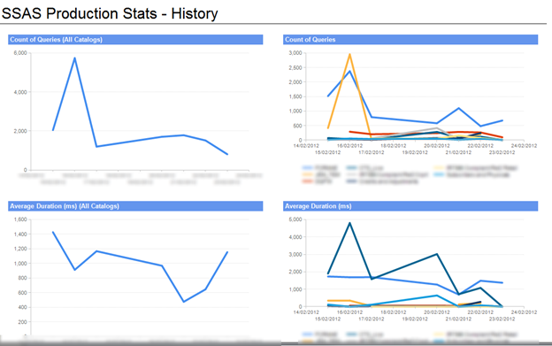
Either way, collecting trace data allows you to create reports like the following, which can be a really nice way to track what’s happening on your servers:

Scripts:

[listyofiles folder=”wp-content/count_queries_scripts”]

What Exists and What is Empty in MDX

After reading my chapter “Managing Context in MDX” in MVP Deep Dives vol2 I noticed that I should have probably discussed one extra topic – the difference between cells which cannot exist, and such which can, but are empty.

The basic idea is that in SSAS cubes we have the notion of empty space. However, there is an important difference between empty intersections which are possible but result in nulls when queried and “impossible” intersections between hierarchies in the same dimension.

If we look at the Date dimension in Adventure Works we can see that we have month and year attributes. Months in 2007 appear only with the year 2007 in the dimension. Therefore, the combination between January 2005 and CY 2007 is not possible and consequentially it does not and cannot exist in our cube. In contrast, if we query for Clothing products in 2007 and we place the Month attribute on rows, we can see that there has been no Clothing items sold in the first few months of 2007:

Here we are dealing with possible, but empty cells – the January 2007 to June 2007 rows show empty intersections in the cube.

Why is this important? Well, it means that if we try to get the number of months with Clothing sales in 2007 with a query like:

we wrongly get 12, not 6. We need a function which can “detect” empty cells – not unnecessarily enforce the current context. An excellent function for this purpose is NonEmpty (or Exists):

Here we get the expected number – 6 (since only 6 months in 2007 have Internet Sales Amount against them).

A similar example can be shown the other way around. The following query returns 37, which is the total number of members of the month attribute with data against them:

This is because the NonEmpty function does not enforce the current context on its first argument and it gives us the members with data only (omitting NonEmpty results in 39, because we have two months with no sales whatsoever). Existing does, so if we add Existing to NonEmpty we get the expected count of 12 (as all months have had a sale in 2007 if we take all categories into account):

Here we eliminated the impossible intersections between months not in 2007 and year 2007.