Cleaning up Hanging Traces with PowerShell

This post is a brief follow-up to my previous post Counting Number of Queries Executed in SSAS. There we saw how we can create and save server-side traces in PowerShell. If you have played with those scripts chances are you have a few hanging traces on your servers. Other possible sources of hanging traces could be Profiler crashes (not on close as it usually cleans after itself), or other applications which do not drop traces they create. To check what’s running on your servers have a look at the XMLA scripts in this blog post by Karen Gulati. It could be nice to have a PowerShell script which drops all traces other than the ones you need. The following script does just that. As it loops over a number of servers you don’t need to install it on multiple machines (provided you have a suitable account). Note that if you are an ASTrace user you may not want to use this as the traces ASTrace creates do not have distinctive names which you can add to the $ExcludeTraces array, so the script would just clean them up as well.

[Reflection.Assembly]::LoadWithPartialName(
    "Microsoft.AnalysisServices") > $null
$SSASServers = @("myserver1", "myserver2")
$ExcludeTraces = @("FlightRecorder", "Important Trace")

foreach($srv in $SSASServers) {
    $conn = 
        New-Object Microsoft.AnalysisServices.Server
    $conn.Connect($srv)

    $traces = @($conn.Traces | 
        where {!($ExcludeTraces -contains $_.Name)})
    $cnt = $traces.Count-1

    while($cnt -ge 0) {
        $traces[$cnt].Drop()
        $cnt--
    }

    $conn.Disconnect()
}

Thanks to Darren Gosbell for his assistance with all things PowerShell 🙂

Is Excel 2013 Power View hurting SSAS?

Since the release of Office 2013 Preview, there has been an awful lot of commentary both in the BI blogosphere and in all media mostly praising the new look and features Microsoft are giving us. I agree that the new suite is getting a much needed face-lift (after all 2007 -> 2010 did not deliver much in this regard), and the mandatory for post-2010 releases “touch-enabled” interface. As a BI guy, the most interesting thing for me in the new Office is Excel, and within Excel, Power View (not completely ignoring the new Pivot Table options like adding new calcs natively, without using the OLAP PivotTable Extensions plug-in).

There are deficiencies in Power View as it stands now (maybe that is why it is an add-in, not enabled by default) but it is a nice data exploration tool which even Stephen Few told me was going in the right direction. It still doesn’t allow us to do things like Top 10, % of Total, etc. which I love in Excel Pivot Tables, but I am hoping that we’ll get all these and more at some point. Together with maps, small multiples and highlighting, Power View does seem like a potential killer application, making other tools like Tableau seem within reach.

However (here we go), in my opinion it has one drawback which really spoils the good things: it doesn’t work on SSAS Multidimensional cubes. I am sure that if someone from the Microsoft SSAS or SSRS teams reads this they wouldn’t be surprised. After all they have heard this numerous times since the release of Power View (even when it was Crescent). Chris Webb wrote about it and caused some stir, it was discussed and the issue was parked as “will be fixed at some point”. I don’t want to resurrect it in its previous format since we now know that a fix is coming (as publicly stated by Microsoft at PASS and other forums), but I would like to point out that last week after demoing Excel 2013 in front of some decision-makers in the organisation I currently work at, I had to answer questions like “So, we can’t use Excel with SSAS at all?” and “Do we have to upgrade all our cubes to in-memory models now?”. This made me think: we can’t cover the whole feature set of SSAS MD in SSAS Tabular, yet we can’t use the new end-user tools on SSAS MD as well. Basically, I am left with one option only – to recommend SSAS MD and Excel Pivot Tables as the only strategy for corporate BI competitive with other vendors like IBM and SAP. Furthermore, since we can’t use DirectQuery on Teradata, I can’t also say that SSAS Tabular is better than SSAS MD as an analytical platform on top of Teradata. Yes, one day when we get it working it will trump all other options, and the Teradata guys I work with are genuinely excited about the future, but it is unfortunately the future, while other options are there now. And the future in IT always looks bright, while the present is a different story altogether.

So, is Excel 2013 Power View hurting SSAS MD? Maybe not directly, but the more we promote Power View (hint: as it’s getting deployed on every workstation we hardly need to promote it), the more we also highlight the deficiencies in SSAS Tabular and make SSAS MD look like the neglected sibling. As for my demonstrations of Microsoft BI, I would probably treat the two components of SSAS – MD and Tabular as two separate stacks. MD – the best out there for corporate BI, and Tabular – the best for team/personal BI, not to be mixed together. To those who can’t wait to get their hands on a powerful, modern analytical tool working on the iPad and use it on a powerful, robust, widely used analytical engine which works on less than terabytes of memory (let me spell it out: Power View +mobile on SSAS MD), we have to tell: “at some point in the future, hopefully”.

PS: Yes, it does sound like yet another whiny post, but we have been waiting for a very long time (in IT-terms) since the inception of Crescent to get this bloody issue fixed and it is hard to imagine mighty Microsoft struggling to catch up behind Cognos (yes, they have mobile – terrible implementation, but works), Tableau (last time I checked they were a tiny company with overpriced products) and QlikView (ugly and slow from what I’ve seen). It’s not like Microsoft weren’t aware of this, and it’s not like it’s happening for the first time – remember how well PerformancePoint did being unable to connect to anything but SSAS MD and having a lacking feature set, plus SSRS to SSAS integration has always been a pain point. The new, quicker, release cycle at Microsoft seems to be delivering the same amount of features in less-complete releases, which doesn’t seem to help with inspiring confidence in its vision and ability to execute. However great these new ingredients are, the dish doesn’t taste that well when some are lacking…tends to get cold quickly too.

Counting Number of Queries Executed in SSAS

When monitoring SSAS we can use a few tools to gain insight into what is happening on the instance. Perfmon is especially interesting as it shows us information about various aspects of the server – we can see memory, disk, CPU and MDX counters out of the box. However, perfmon cannot show us how many queries were run on SSAS – neither per period (e.g. second), nor in total since the service had started. We have another counter, similar to a count of queries – Storage Engine Query : Total Queries Answered. This is not the same as the number of MDX queries answered, as if a query does not hit the Storage Engine (SE), but the Formula Engine (FE) cache instead, it won’t increment the counter. And, if a query needs to be answered by more than one Storage Engine requests, we will see that the counter gets incremented with more than 1.

There are alternatives. We can try using the Query Log server settings and save queries to a database table automatically:

Unfortunately (for us in this case), since the Query Log is typically used for Usage Based Optimisations (UBO), it also shows SE requests, not the actual MDX queries issued. Hence, it suffers from the same drawback as the perfmon Total Queries Answered counter.

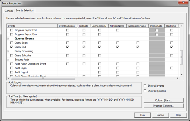
The other alternative which comes to mind is SQL Server Profiler. After all it allows us to see what queries get sent to the server, along with lots of other useful information. If we are interested in the count of queries only, we can capture a trace which includes only the Query End event. Why not Query Begin? Well, we can’t see some possibly interesting numbers before the query has been executed, for example the Duration of each query. If we capture only Query End we get exactly what we need – one event per query. We can also capture Error events to check if things go wrong.

A typical Query End-only trace looks like this (all columns included):

As we can see above, we get the actual query in the TextData column, the User Name, Application Name, Duration, Database Name – all very useful properties if we want to analyse the load and the performance of our server and various solutions. While the information looks great on screen, having it in a database table would enable us to do what we (BI devs) like doing – play with the data. Only this time it’s our data, about our toys, so it (at least for me) is twice as fun.

A SSAS trace can be run on the server without Profiler – the term for it is a “server-side trace”. Unlike SQL Server RDBMS traces, a SSAS server-side trace cannot directly log its output to a SQL Server table. Luckily, we can write the results in a “.trc” file, which in turn can be imported into a SQL Server table with a few lines of code.

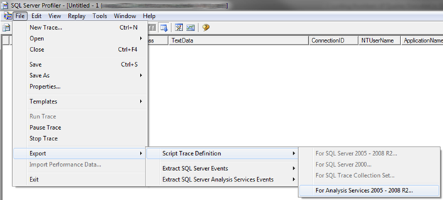
To create a server-side trace we can first export the trace definition to an XMLA file from profiler:

The XMLA file we get looks like this (all scripts are attached to the end of this post):

If we remove the first line (?xml version…), we can run this and it will create a trace on the server. This trace is useless to us because it does not write its output anywhere. To fix this we can add a few settings like this:

Note that I have changed the Name and ID of the trace to be more user-friendly, and I have removed the Filers section, as well as the first line. Now the script can be used to create a trace. To delete the trace we can use:

And to list all running traces on a SSAS instance:

Note that by default SSAS is configured to run Flight Recorder, which uses a trace to capture events happening on the server (thanks to Dan English for suggesting this clarification). The trace may appear with ID and Name of FlightRecorder. You should not tamper with the trace manually. If you want to stop it, which is a performance recommendation from the SSAS Performance Guide, you should disable Flight Recorder from the SSAS server properties (click for a larger version):

Now, armed with all these scripts we can effectively manage traces on our instances. The only problem we have not resolved so far is exporting the trc file created by our create trace XMLA command to a database table. This can be easily done in a .NET app, or in PowerShell. The ps_trace_copy_to_table.ps1 PowerShell script does the following (thanks to Darren Gosbell for creating the initial version).

  1. Copy the trc file with another name for further processing
  2. Delete the trace form the server
  3. Delete the trace file
  4. Start the trace on the server again
  5. Export the copied trc file into a SQL Server table
  6. Run a stored procedure moving the data from the SQL Server table to another SQL Server table which contains all trace data

We delete->create the trace because otherwise we cannot delete the trace file. The last step runs a stored procedure which moves the data from the table we imported into to another table because the first (landing) table gets re-created every time we import into it and the trace data cannot persist in it.

Note that there is some exception handling implemented in this script (try/catch/finally blocks). If you are using an old version of PowerShell, it is possible that you may have to remove the exception handling statements as they were not supported. I have attached a sample script which excludes them (ps_trace_copy_to_table_no_exception_handling.ps1).

Finally, we can run this script through SQL Server Agent on regular intervals. SQL Server Agent allows direct PowerShell script execution, so this is very easy to set up and can be scheduled to run recurrently every X minutes/hours/days.

A small note: you may notice that some rows in the database table contain events with an Event Class <> 10 (10 is Query End) and NULLs in most columns. These are trace-related events and can be ignored (e.g. your stored procedure moving the data form one table to another can skip such rows).

There is also another way to achieve the same outcome. As a part of the Microsoft SQL Server samples you can download a utility called ASTrace. You will have to download and compile it, but after that you can run it as a Windows service and it will capture the trace events as they happen and write them directly to a SQL table. The Server -> File -> Table changes to Server -> Table. Also, you don’t need to move the data from one table to another. The drawback is that you have an additional service on your server. You may or may not be able to run it (depending on your organisation’s security policies and admin practices), and while it is open source, it is not officially supported by Microsoft.

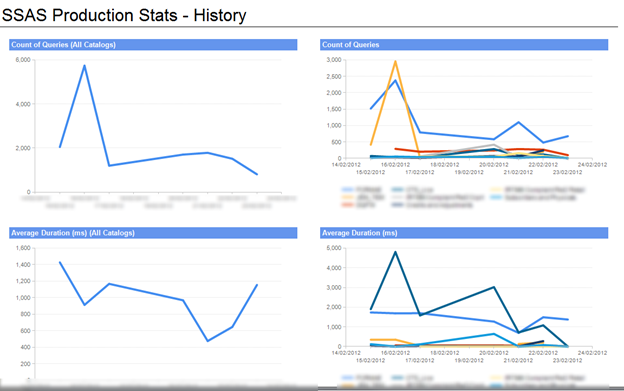
Either way, collecting trace data allows you to create reports like the following, which can be a really nice way to track what’s happening on your servers:

Scripts:

[listyofiles folder=”wp-content/count_queries_scripts”]

What Exists and What is Empty in MDX

After reading my chapter “Managing Context in MDX” in MVP Deep Dives vol2 I noticed that I should have probably discussed one extra topic – the difference between cells which cannot exist, and such which can, but are empty.

The basic idea is that in SSAS cubes we have the notion of empty space. However, there is an important difference between empty intersections which are possible but result in nulls when queried and “impossible” intersections between hierarchies in the same dimension.

If we look at the Date dimension in Adventure Works we can see that we have month and year attributes. Months in 2007 appear only with the year 2007 in the dimension. Therefore, the combination between January 2005 and CY 2007 is not possible and consequentially it does not and cannot exist in our cube. In contrast, if we query for Clothing products in 2007 and we place the Month attribute on rows, we can see that there has been no Clothing items sold in the first few months of 2007:

Here we are dealing with possible, but empty cells – the January 2007 to June 2007 rows show empty intersections in the cube.

Why is this important? Well, it means that if we try to get the number of months with Clothing sales in 2007 with a query like:

we wrongly get 12, not 6. We need a function which can “detect” empty cells – not unnecessarily enforce the current context. An excellent function for this purpose is NonEmpty (or Exists):

Here we get the expected number – 6 (since only 6 months in 2007 have Internet Sales Amount against them).

A similar example can be shown the other way around. The following query returns 37, which is the total number of members of the month attribute with data against them:

This is because the NonEmpty function does not enforce the current context on its first argument and it gives us the members with data only (omitting NonEmpty results in 39, because we have two months with no sales whatsoever). Existing does, so if we add Existing to NonEmpty we get the expected count of 12 (as all months have had a sale in 2007 if we take all categories into account):

Here we eliminated the impossible intersections between months not in 2007 and year 2007.

SSAS Locale Identifier Bug

These days I have two little problems with SSAS. One is really small – I really don’t like how the Process dialog in BIDS (2008 R2) stays blank during the process operation and how I need to click on “Stop” after it finishes. The fact that such a bug had gotten into the product and has survived for so long when it happens 80-90% of the time doesn’t speak very well for the QA process at Microsoft. However, I can understand that the impact of this bug would have been deemed very insignificant as it impacts developers only and does not prevent them from doing their job. By the way, if you are also annoyed by the blank process dialog in the latest version of SQL Server, you will have to wait until the next release (2012) until you get a fix:

http://connect.microsoft.com/SQLServer/feedback/details/536543/ssas-process-progress-window-blank-no-details

The other bug is far more significant. It not only impair developers’ ability to build some features, but is also highly visible to all Excel users. However, it is hard(er) to reproduce:

http://connect.microsoft.com/SQLServer/feedback/details/484146/getting-an-error-when-trying-to-browse-a-cube

Still, it seems like developers from {[World].[Countries].Members}-{[World].[Countries].[USA]} hit it all the time. I am speaking about the Locale Identifier bug. The most common occurrence is when drilling through to detail in Excel. After the drill-through action has been initiated, Excel shows a message box with a message talking about the XML Parser and how the Locale Identifier cannot be overwritten –

“XML for Analysis parser: The LocaleIdentifier property is not overwritable and cannot be assigned a new value.”

The cause is simple (as confirmed by the SSAS team at Microsoft and Akshai Mirchandani in particular): once we open a session we cannot overwrite the locale. The mystery is around the cause for Excel to do something like that. Noting that Excel is not the only offender, as I have also seen the same error message thrown by SQL Server Profiler, and Chris Webb has seen it with the Cube Browser in BIDS:

http://connect.microsoft.com/SQLServer/feedback/details/484146/getting-an-error-when-trying-to-browse-a-cube

Since the bug has been reported to Microsoft, we are now hopeful that a fix will appear at some point. Until then you can try the following workaround, courtesy of my friends and former colleagues Matthew Ward and Paul Hales:

– Switch the Windows Region and Language Format in Control Panel to English (United States):

– Switch it back to whatever it was before

Now the “bug” should be fixed for that machine. For example, I had my new Windows 7 workstation configured to use Australian formats. After I got the Locale Identifier error message in Profiler, I switched the formats to USA. The bug disappeared and I could profile SSAS. After that I switched Windows back to the original English (Australia) format…and nothing broke. I could still use Profiler and drill-through in Excel.

Another notice. Greg Galloway has released a new version (0.7.4) of the OLAP Pivot Extensions add-in for Excel. In case you have been experiencing a Locale Identifier problem in SSAS while using older versions of the add-in, please download the new one and let Greg know (e.g. on the discussions page on CodePlex) if the new release fies your problem.

Thanks to everyone involved in confirming and testing different fixes. Ideally, I would like to see Microsoft fixing this on the server side of things which would allow us to easily patch up all existing systems exhibiting the problem.

Since all Microsoft Connect item related to this bug have been closed, I opened a new one, so you can vote in order to prioritise this issue:

https://connect.microsoft.com/SQLServer/feedback/details/721372/locale-identifier-bug

Note (2012-03-21): The issue seems to be with Windows Vista+ as confirmed by Michael Kaplan – http://blogs.msdn.com/b/michkap/archive/2010/03/19/9980203.aspx

SSAS: Multiple SQL Queries in ROLAP Mode

Just recently I was working on a project where I had to build a SSAS ROLAP cube on top of a badly built data mart. Badly built in this case meant one where we encounter multiple referential integrity (RI) issues. Most importantly, the designers ignored the very basic principle that all dimension keys for each row must be present in the respective dimension tables. When in MOLAP mode, SSAS checks for such mismatches during processing. However, when a partition is in ROLAP storage mode, we don’t get a notification that anything is wrong and the cube processing operation succeeds. This situation has some consequences during execution time and I will try to illustrate those in this post and show a solution. Before I begin, I must say that if it wasn’t for Akshai Mirchandani’s (from the Microsoft SSAS dev team) and Greg Galloway‘s help, I would have probably spent quite some time figuring out what is happening. Thanks to them the problem got solved quickly and I got to understand the reason for what is happening.

In terms of set-up, I created two tables in SQL Server: Dim and Fact. The Dim table contained two members A and B, with keys of 1 and 2. Initially, the Fact table had two rows referencing the Dim table – Dim keys of 1 and 2, and a measure column called Amount with 1.0 and 2.0 as the amounts corresponding to A and B. No issues here. After that I created a SSAS solution, corresponding to this simple dimensional model. I switched the partition storage for the cube to ROLAP and processed the SSAS database. After that I ran the following query, which I used for all subsequent examples:


The result was as expected:


At the same time I had a SQL Server Profiler trace running, which showed:


We can see that SSAS has executed one SQL query retrieving data from the fact table. Nothing unusual thus far.

To spoil the party, I added one more row to the fact table with a dimension key of 3 and Amount of 3. Since I did not add a row in the dimension table with a key of 3, this broke the rules and if I had a foreign key constraint implemented between the fact and the dimension tables I would not have been able to do this. After cleaning the SSAS cache, I ran my query again. The result:


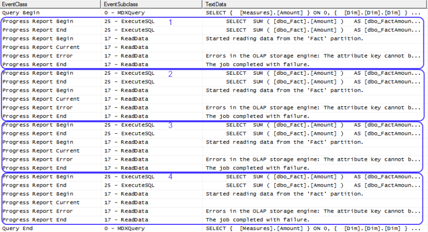
The actual error was, of course, a missing key. I was not surprised when I saw this on my original project. However, looking at Profiler we see a “weird” sequence of events:


SSAS runs multiple queries which result in errors. In this case we can see four of these ExecuteSQL events. All of them are followed by an error in a ReadData event. In this particular case we can see only four ExecuteSQL events. In the real-world, this scenario can get multiple times worse (in my case we saw 4667 queries run against the relational database in a few minutes) leading to a really significant drop in performance.

So, what is happening? According to Akshai, SSAS encounters an error while dealing with the results from the initial SQL query and is trying to recover by sending more queries. In some cases this can result in getting the error in the result set only for some cells.

Luckily, there is an easy way out of this situation (thanks to Greg for providing the tips). SSAS can automatically create an “unknown bucket” for each dimension and can assign to it all measure values which do not correspond to a dimension member. To get this result, we must ensure that each affected partition’s error configuration is set to something similar to:


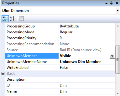
Note that the KeyErrorAction is ConvertToUnknown, not DiscardRecord (which is the alternative). This must also be coupled with setting up each “incomplete” dimension to include an Unknown member:


It does not matter whether the UnknownMember is Visible or Hidden, as long as it is not None.

Back to our scenario. After setting these properties on the dimension and the partition I processed the SSAS database again and executed the query. The result:


and the profiler trace:


As we can see we eliminated the multiple queries. If we do not want to see the Unknown amount in the cube we can use a scope assignment:


Coupled with making the UnknownMember Hidden, we can completely obliterate traces of our underlying RI issues. Unless our users check the numbers, but then we can blame whoever designed the datamart! 🙂

Alternate Ordering of Attributes in SSAS

Sometimes we need to display attribute members in SSAS in a different order than the order of its name or key. For this purpose we have the option to use one of its attribute’s name or key. However, in some cases changing the order may break some calculation logic which depends on the initial order. The new ordering may also be inconvenient for writing MDX as using some functions of the language is easier (at least conceptually) when thinking of sets in ascending order. The best example which we can use to illustrate this problem is the Date dimension. While in most, if not all, cases the Date dimension is ordered in ascending order, sometimes users prefer to see the most recent date first and request us to change the order to descending. Doing so invalidates many time intelligence calculations like rolling and parallel periods, etc. Furthermore, fixing those requires inverting numbers to negative, or avoiding the use of functions like ClosingPeriod. All in all, a “small” change can lead to a big problem. We can, however, accommodate our ignorant users (which unknowingly get the benefit of reading default time series charts backwards – from right to left – when dragging-dropping descending dates in Excel, for example) without changing too much in our scripts. A little trick in the modelling can help and it is the reason for writing this post.

Let’s have a look at a simple Date dimension with one attribute – Date. Nothing unusual, with the Date being ordered by its Key (integer in this case) and with a name coming from another column in the Date table – DateName. When we create a simple slice in Excel we get the following:


Now we create a measure Rolling 3 Days Amount, which sums the last 3 days’ amount:


The MDX for this calculation is:


If we simply invert the order of the Date attribute by ordering it by another column in our Date table, which contains DateKey*-1 and refresh the Excel pivot table we get the following:


This is simply incorrect. A relatively small change in the MDX script can help us with this issue (e.g. changing the Lag to Lead), however in many cases we do not want to rebuild all the measures. Luckily, we can employ a different tactic. Instead of changing the script, we can change the structure of our dimension by adding an additional attribute which is not exposed to the users. (i.e. is hidden). This attribute will be based on the same column we use for our Date, but will not be ordered by the descending column. We can rename the original attribute (the one exposed to the users) to something like Date Desc, or a more user-friendly option, and hide the new one:


Everything else stays the same – our cube script does not need to be adjusted and its logic is correct:


A different approach could be to leave the old attribute named Date, so there is no change necessary in case of reports depending on the naming. This, however, requires a change of the cube script, which can be easily performed with using the BIDS Replace functionality (e.g. Ctrl+H).

Note that for this approach to work we need to make sure that the attribute exposed to the users is the dimension key attribute as changing its current member results in an (infamous) attribute overwrite where its related attributes, which are above it in the relationship chain) also change. If we expose the non-key date attribute our MDX logic will break as the changes to its current member will not affect the attributes below it (actually, it will set them to their All member).

Building a Date Table

Date tables in themselves are nothing new. Every data warehouse and business intelligence project includes one of those and typically it is one of the first tables which we find on our list of implementation tasks. Surprisingly, however, I am finding that in many implementations the omnipresent date table cannot support some analytics. In this post I will outline a few considerations which we need to take into account when building date tables in general, and some which apply specifically to SSAS.

UPDATE (9th October 2011): If you are a PowerPivot user (or would not mind using an OData feed) there is a simple way to get a date/calendar table as there is a free one available on the Azure DataMarket. I recently blogged about this new project in my Introducing Project DateStream (CodePlex) post.

UPDATE 2 (16 October 2011): John Simon recently published a nice T-SQL script which can be used to create and populate  a date table on his blog. Have a look if you need one!

Grain, Key and Format

In general, date tables are on a daily/date grain. This is because the lowest level of reporting we need to do is very often on full days. Even if we need to analyse on time intervals smaller than a day, we should still build a Date and a Time table to support this. Why? Because if we pack it all in the same table we end up with too many rows and this is something we typically want to avoid in any dimension. As we have a row per day, one of our columns is inevitably based on the calendar date. It is also typically the dimension key. As with all other dimension tables, we need to be able to join the table to our fact tables and this is done on our key. To keep our fact tables as small as possible, we need the smallest possible data type for our keys, and in the case of a Date this is usually an integer. However, unlike with other dimensions, we do not have to have a meaningless integer for our surrogate key because it does not give us any advantage. It is very easy to convert between a datetime and an int and in SQL Server datetime is 8 bytes, while int is 4. In SQL 2008+ we have another type suitable for our date table key – date, which is 3 bytes. However, for compatibility reasons, it is frequently better to stick to an int. Luckily, we also have the very convenient ANSI/ISO 8601 standard to follow in order to make our integer dates easier to work with. If we do encode them with the YYYYMMDD format, (thus the 15th of January 2011 becomes 20110115), we can easily sort on the column and compare two dates with the standard > and < operators. Additionally, we also escape the ambiguities around date formats in the USA and the rest of the world.

Attributes

Building the date key column is a good start but to allow for better analytical capabilities we need to add other attributes. As in most cases we need to analyse our data not only on days, but also on larger intervals (e.g. Months, Quarters and Years), we need to add columns for each of them. A typical requirement is to support both Financial and Calendar date hierarchies. As with dimensions it is ok to have many columns, we can add one for each combination of the type of calendar and period (e.g. FinancialMonth and CalendarMonth, FinancialQuarter and CalendarQuarter, etc.). Other interesting attributes we may want to have materialised in the table are the likes of Weekends, Public Holidays (even though we need to maintain these), Solstice/Equinox and PhaseOfMoon (thanks for Thomas Kejser for mentioning these in an online conversation recently). Basically, for a fully functional date table we need to consider anything which could be of business value without going to extremes.

Of course, when working with SSAS we also want to have an integer key for each attribute and possibly a common name for it. This multiplies the number of columns we need by two – one Id and one Name column for each of the attributes we have decided to implement. Some attention needs to be spared when determining the formats of each attribute Id. If we are to be building a hierarchy out of a collection of attributes we want those to form a nice natural hierarchy. That is – each child member should not have two parents with different Ids. To illustrate the concept, let’s consider two different months – January 2011 and January 2012. While they are the first month of the calendar year, they represent different entities when reporting. We do not aggregate data to January only, but to January in each respective year. Therefore, if we were to write a SQL query to get data for January 2011 and our Ids for both of these members are 1, we would also need to use the Year attribute to get the values we need. Effectively, our hierarchy would have two children with identical Ids of 1 with different parents (with Ids of 2011 and 2012). This is a particular problem when working with SSAS as it definitely prefers unique Ids for each separate attribute member. There is a very easy solution – we can include both the Year and the Month number in the MonthId. In our case, January 2011 gets an Id of 201101 and January 2012 – 201201. Now we don’t have the same issue. Similarly, we must pay attention when we construct the Ids of other attributes which participate in our hierarchies like Quarter (YYYYQQ) and Half Year (YYYYHH).

Weeks

The week is a special case in the calendar. While we can say that Days roll up to Months, which roll up to Quarters, which in turn roll up to Half Years and Years, Weeks are a different story. If we are not using a special calendar like a 4-4-5 calendar, we are dealing with a real-world entity, which does not naturally belong to only one larger period. In most cases we do not have to worry about the week falling between Day and Month as business understands that this is not a very easy to work with hierarchy. However, business users very often are ignorant about the fact that weeks do not roll up nicely to years, too. We can again read ISO 8601, which also deals with the Week->Year problem. Basically, the ISO has come up with a simple solution – if we have a week which has dates in two years, we count it towards the year which contains more dates (or, the year which contains the Thursday of the week). Why is this important? Well, we can simply split a week in two, however, this means that certain weeks in our table contain less than 7 days. If we compare such weeks with a Weekly Growth calculation we will notice a problem – the amounts aggregated to them are smaller than usual. Similarly, on a graph showing weekly amounts, we have a dip as the two parts of the same week are plotted as separate points. If the users do not care, then it is not a problem, but it is something we should consider and ask about when building the week attribute in our date table.

Ranges

The date table has a limited amount of rows and we have to make a decision on how many are enough. Some developers build date tables with ranges all the way from 1900 to 2100, or even further. As we have roughly 365.25 days per year (note how 1900 is not a leap year, not is 2100 – something Excel doesn’t know), for 10 years of data we end up with ~3652 rows. With 100 years we have 36525 rows. It is quite doubtful that a data warehouse will contain data for all these years. In most cases it contains a bit of historical data and is designed to keep data for another 20-50 years. To optimise the performance of the queries using the date table it is a good idea to have a dynamic range of dates. In our ETL we can easily keep expanding the range as needed, or collapse it if we ever purge fact data. One thing which is often overlooked when picking the date range is the fact that many times queries depend on the completeness of the date range. A major mistake, which we must avoid are basing the date table on fact data and allowing gaps in the range, and having incomplete top-level periods.

The first problem is easy to explain. Zealously trying to keep the date dimension as small as possible by reducing the number of days (i.e. rows) to only the applicable ones for our fact data can introduce gaps in the overall table. In example, if we have no data for 26th of January because our business was closed for Australia Day, and we “optimise” the date table to exclude this day from the date table, all analytics which depend on counting the number of dates in January will be skewed. An average calculation doing Sales/NumberOfDaysPerMonth will divide by 30, not 31. One of the reasons for having a date table at the first place is to avoid such problems. Hence, gaps in the date table must be avoided.

Secondly, we must also ensure that all top-level periods (i.e. Year usually is the top level in the Calendar Hierarchy) must be also complete. It is not acceptable to cut off the date range with a month, so we have a constant number of dates. Even if our fact data is implemented over a fixed window of 24 months (rolling), we should not do the same with the date table. In example, if we are in September 2011 and we have fact data for 24 months prior to this (e.g. September 2009 – September 2011), the date table should also include data for months prior to that (e.g. January 2009 – September 2011). The reason is the same as before – all calculations doing Amount/NumberOfPeriodsWithinAPeriod would be wrong for 2009. Furthermore, if we use something like window functions in SQL partitioning by year and counting the months within the period to compare equivalent ones will be incorrect. The first month of 2009 would be September and the first in 2010 – January. Because of such issues, it is best to keep all top level periods complete. A solution could be removing data from the date table once we are not interested in the complete top level period. In the case of the 24 rolling months, we can remove all of 2009 with all its periods/rows once we move to 2012 and we are interested in January 2010 – January 2012.

In SSAS all date functions like ParallelPeriod and ClosingPeriod work with relative periods. To get the ParallelPeriod for January 2010 in 2009, SSAS will determine that January 2010 is the first month in 2010, go back to 2009 and pick the first month there. If the first month is September 2009, we will get that returned.

Unknowns

As with other dimensions, we should also have an Unknown member in the date dimension. While with all other dimensions we usually pick a value like -1 for the Unknown member Id and Name of “Unknown”, with a date table things a slightly different as we often have columns which are some sort of a date/time data type and we cannot cast -1 to a date in a meaningful way. Therefore, in many cases we can pick a complete outlier, like 19000101, which we use for storing Unknowns. Depending on the scenario, we may not need to do that, but if we do, there is nothing wrong with doing that as long as we make sure that it is clear that it is a special case. If the data starts in 2001 and we pick 20000101 as an unknown value many users will be wondering why there is some data against that date.

Conclusion

The best date table is the one we don’t notice and take for granted. Given that it is not something that changes at all, the structure of the date table is the one common over many different implementations and whether in SQL Server, SSAS or PowerPivot, the fundamentals stay the same. It can be shared and is part of the base of virtually every BI solution. It, unfortunately, is built wrong very often, thus severely impairing the capability of the system it is a part of. With the arrival of self-service BI I could imagine an increasing need for practical advice on this specific data modelling technique and I hope this article helps with delivering a bit of it.

SSAS Myths Dispelled

This post is an attempt to dispel a few myths which seems to get repeated over and over among SSAS developers. While the truths are nothing new and have been documented in multiple sources like BOL, SQL CAT whitepapers, books and blog posts, they seem to consistently escape the attention of the wider public.

1 SSAS pre-aggregates data by default

While it is true that SSAS can pre-aggregate data this does not happen by default. SSAS compresses data, indexes data and caches data but it does not pre-aggregate data unless we define aggregations. When I am saying pre-aggregate I mean that SSAS does not automatically know what the Internet Sales Amount for Australia in 2007 is. It needs to get the leaf-level data and sum it up; unless we have built an aggregation on Country and Year for the partition containing the Internet Sales Amount measure. In that case the data is pre-aggregated and ready for retrieval.

2 We can emulate in MDX at no cost Enterprise Edition functionality in Standard Edition

Well, we can’t. We can emulate certain features like LastNonEmpty aggregation functions for example, but it comes at a cost. The cost usually relates to Storage Engine (multi-threaded) vs Formula Engine (single-threaded) execution.

3 SSAS is always faster than SQL Server RDBMS

While it is true that SSAS is faster than SQL Server RDBMS in many cases, this does not always hold true. A particular area in which the relational engine beats SSAS is the retrieval and processing of low-level granular data. SSAS usually beats the RDBMS when it comes to ad-hoc access to aggregated data.

4 MOLAP is always faster than ROLAP

If you read SQL CAT’s “Analysis Services ROLAP for SQL Server Data Warehouses” whitepaper you can see that after careful tuning ROLAP can be faster than MOLAP. Not always, but sometimes – enough to claim that it is not true that MOLAP is always faster than ROLAP. This ties a bit to the previous myth and proves that a well tuned RDBMS can perform very well with aggregates.

From the paper:

“At last, SQLCAT’s redesign and optimization efforts paid off. The ROLAP cube was finally ready for performance testing, and thanks to the amazingly fast performance of the relational SQL Server engine on top of a super-fast storage subsystem, the results looked better than expected. To everybody’s surprise, the ROLAP cube outpaced the MOLAP cube in 45 percent of all queries right from the start (see Figure 14). Only 39 percent of the queries showed substantially slower response times in ROLAP mode (more than twice the amount of MOLAP time) and 16 percent showed moderate performance degradation (less than twice the amount of MOLAP time).”

5 Usage Based Optimisations do not work well

In SQL Server Analysis Services 2008 the Usage Based Optimisation (UBO) algorithm has been redesigned. Now it works, and it works well. It does not create redundant aggregations and in general performs much better. Building UBO aggregations has always been recommended by Microsoft and even more so now.

6 Rigid attribute relationships boost performance

Whether an attribute relationship is Rigid or Flexible does not actually improve performance at all. Not query performance. A wrong choice here only affects processing of partition indexes. If an attribute relationship is static, setting it to Rigid means that you do not have to process partition indexes when you update the dimension. This is all the benefit you get from Rigid relationships. Going too far and marking changing relationships to Rigid may have a very negative impact as a change will prompt a complete process of the partition data and indexes, which will take much longer than updating just the indexes. Either way, there is no difference during query execution.

7 MDX and DAX are hard

I believe that this particular myth stems from the fact that we get to compare MDX and DAX to sweet and fluffy languages like SQL and C#. It all depends on the vantage point. Take the following “Hello world!” program in Malbolge for comparison purposes:

(‘&%:9]!~}|z2Vxwv-,POqponl$Hjig%eB@@>}=<M:9wv6WsU2T|nm-,jcL(I&%$#”
`CB]V?Tx<uVtT`Rpo3NlF.Jh++FdbCBA@?]!~|4XzyTT43Qsqq(Lnmkj”Fhg${z@>

MDX is not all that bad from a Malbolge developer’s point of view, is it?

Custom Groups in Excel 2007 – Error

I just finished digging around a particular issue with Excel 2007 (some versions) and SSAS Pivot Tables. In brief, the issue was that a user could not use the custom groups functionality which Excel provides because she got an error saying:

“The query did not run, or the database table could not be opened. Check the database server or contact your administrator. Make sure the external database is available and hasn’t been moved or reorganized, then try the operation again.”

I added her to the server administrators, but the message persisted. After profiling I noticed that the MDX generated by Excel 2007 for this operation read:

CREATE SESSION CUBE [Cube_XL_GROUPING0] FROM [Cube] ( DIMENSION [Cube].[Agency].[Agency Hierarchy] HIDDEN AS _XL_GROUPING0,DIMENSION [Cube].[Agency].[Flag],DIMENSION [Cube].[Agency].[Region],DIMENSION [Cube].[Collection].[Application],DIMENSION [Cube].[Collection].[Application Code],DIMENSION [Cube].[Collection].[Data Collection Code],DIMENSION [Cube].[Data…

Error: “Parser: The syntax for ‘DIMENSION’ is incorrect.”

I have highlighted the problematic part – the MEASURE part of this expression was missing. A correct MDX statement issued by another instance of Excel 2007 running on a different machine showed:

CREATE SESSION CUBE [Cube_XL_GROUPING1] FROM [Cube] ( MEASURE [Cube].[Value – Data Integer Quarter] HIDDEN,MEASURE [Cube].[Value – Data Integer Semi] HIDDEN,MEASURE [Cube].[Value – Data Integer Annual] HIDDEN,MEASURE [Cube].[Value – Data Integer Month] HIDDEN,MEASURE [Cube].[Value – Data Real Quarter] HIDDEN,MEASURE [Cube].[Value – Data Real Month] HIDDEN,MEASURE [Cube].[Value – Data Real Annual] HIDDEN,MEASURE [Cube].[Value – Data Money Semi] HIDDEN,MEASURE [Cube].[Value – Data Money Month] HIDDEN,MEASURE [Cube].[Value – Data Real Semi] HIDDEN,MEASURE [Cube].[Value – Data Money Quarter] HIDDEN,MEASURE [Cube].[Value – Data Money Annual] HIDDEN,DIMENSION [Cube].[Agency].[Agency Hierarchy] HIDDEN AS _XL_GROUPING0,DIMENSION [Cube].[Agency].[Pub Pte Flag],DIMENSION [Cube].[Agency].[Region],DIMENSION [Cube].[Collection].[Application],DIMENSION [Cube].[Collection].[Application Code],DIMENSION [Cube].[Collection].[Collection Code],DIMENSION [Cube].[Element].[Common Name],DIMENSION [Cube].[Element].[Data Element Code],DIME…
Here we have the cube measures as a part of the CREATE SESSION CUBE statement and this makes it a valid one. The reason for this seems to be the fact that all the physical measures in the cube were hidden and only one calculated measure was shown to the users. Excel (2007 Enterprise) seemed unable to find them, so the fix was easy – creating a visible dummy physical measure and using a scope assignment to make it work like the calculated one. Now Excel merrily creates valid MDX and my user is happy.

I understand this will be a very rare problem, but it takes some time to investigate, so I hope the post may help someone out there.